How To Interpret RT-qPCR Results
by Adriana Gallego, Ph.D.

by Adriana Gallego, Ph.D.
You have just finished your real-time quantitative reverse transcription PCR or RT-qPCR experiment. Now what? How do you analyze your data?
To analyze your qPCR data, you will need some prior knowledge about the methods to differentiate the expression of the target gene from the rest of the gene.
The internet is filled with different methods, procedures, and workflows that can overwhelm you during data analysis, especially if this is your first time with RT-qPCR. This article is going to dive into some tough concepts, each getting a little trickier. So, I will break down the three areas of qPCR interpretation that we’re going to detail in this article:
Please note that in this article, we will refer mainly to qPCR as a placeholder term for both qPCR and RT-qPCR. Occasionally, we will discuss the two methods interchangeably. Either one can work for this article in most every occasion mentioned.
This article also offers different online calculators to obtain Ct values and gene expression ratios so check it out here.


Absolute vs. Relative Quantification
Methods for relative quantification
Calculating Ct values when using the Livak method
Calculating Ct values when using the Pfaffl method

Figure 1. Example of a qPCR or RT-qPCR chart with the six main elements labeled.
When reviewing articles about qPCR data analysis, one common thing we have discovered is that the qPCR chart is not explained in detail.
During RT-qPCR, the accumulated target DNA (expressed as fluorescence) is detected and measured as the reaction progresses, and this information is plotted on a qPCR chart.
The qPCR detection methods use a fluorescent signal to measure the amount of DNA in a sample. The fluorescence can be expressed as “R” (raw fluorescence) or “Rn “(normalized reporter). The Rn value is a value calculated by dividing the fluorescence of the reporter dye (e.g., SYBR Green) by the fluorescence of a passive reference dye (ROX).
The fluorescence, expressed in Rn or R values, is plotted on the Y axis.
There are six main elements on the qPCR Chart (refer to figure 1 as a reference):
The Ct also has alternative names such as Cq (quantification cycle) and Cp (cycle point).
Ct is defined as the intersection between an amplification curve and a threshold line, and it is a relative measure of the concentration of the target in the PCR reaction. The Ct values are plotted in the X axis.
The baseline measurement in qPCR is the level of signal during the first 5-15 cycles. During this time, there is little change in fluorescence, which means the signal detected establishes the level of background signal detected.
As qPCR measurements are based on amplification curves, they are sensitive to background fluorescence. This background is also known as “fluorescence noise.” There are different causes, such as light leaking into the sample well and plasticware.
Generally, a low background is expected when compared to the amplified signal of your target sequence. To separate the background fluorescence from the amplified signal for your target sequence, researchers establish a baseline. To establish a baseline, use the fluorescence intensity during early cycles (5 to15) to set up a constant and linear component of the background fluorescence. Fortunately, many qPCR machines automatically calculate the baseline.
The threshold is the point of your qPCR reaction where a significant increase of fluorescence above the baseline is detected.
Since the baseline is set at the limit of detection for the qPCR machine, the measurements at this point would be very inaccurate. Therefore, the threshold is established when a significant signal is detected above the baseline. The qPCR threshold is positioned sufficiently above the baseline to be confident about the amplification curve data.
The qPCR amplification curve represents the accumulation of DNA templates over the complete duration of the qPCR experiment.
The qPCR plateau is the decrease in the rate of accumulation of the DNA molecules, which is seen in later PCR cycles.
PCR efficiency is a ratio calculated by taking the number of amplified target DNA molecules at the end of the PCR cycle divided by the number of DNA molecules present at the beginning of PCR.
The efficiency should be between 85-110% to be acceptable. An efficiency higher than 100% could be explained by an excess of template or the presence of inhibitors. These conditions produce a lower slope in the data that leads to an efficiency over 100%. Furthermore, this efficiency is also dependent on the master mix performance, sample quality, and the assay.
PCR efficiency is incredibly important because it affects Ct values and therefore, all the conclusions you can infer from the RT-qPCR data. For instance, a lower efficiency will yield different Ct values, which can produce false positives.
The efficiency is calculated based on serial dilutions of a known amount of DNA template. With these serial dilution samples (SDS), you will get the Ct values after the qPCR ends. Ideally, you should perform three technical replicates (qPCR reactions) per each SDS.
Let's look at how PCR efficiency is calculated:
Prepare the samples with the chosen serial dilutions. In our case, we used the stock or original sample and dilutions from this of 1/10, 1/100, 1/1000, 1/10000.
After running your qPCR for these dilution samples, you will obtain the Ct values for each of your three technical replicants.
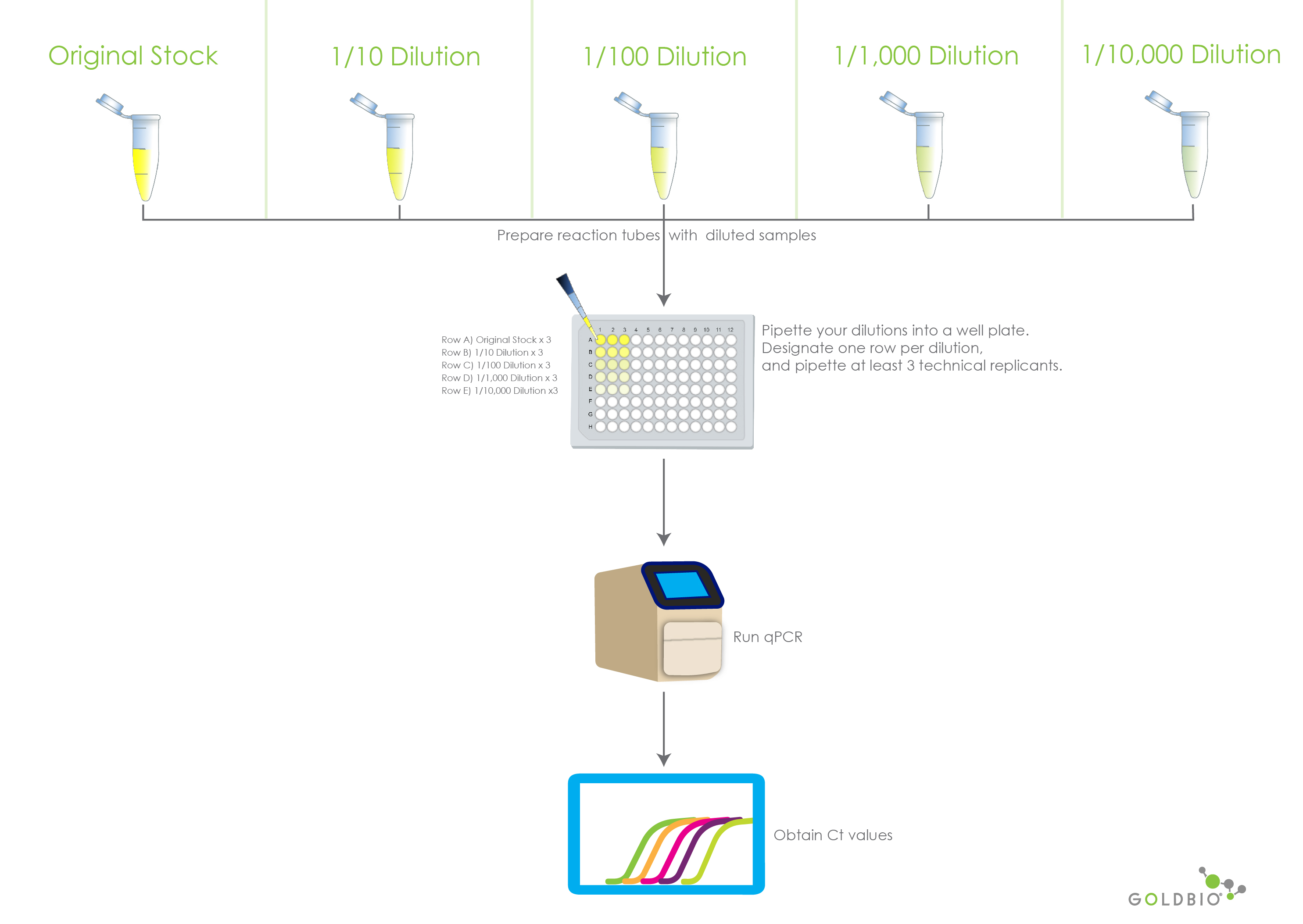
Figure 2. Illustrates the preparation and reading of qPCR and RT-qPCR serial dilutions. The Ct values will then be used to calculate PCR efficiency.
Fill out the table below with the following information. We’ll
take you through step-by-step in the sections below.
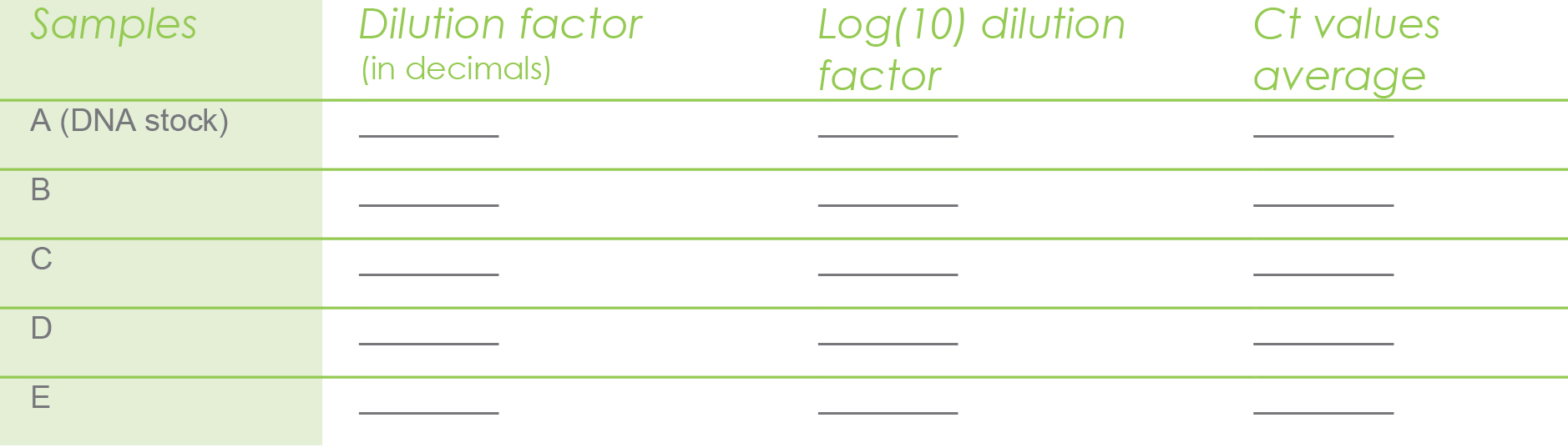
To complete the table above, we need the dilution factor, which is very easy to determine. This is the chosen serial dilutions. In our case we used 1/10, 1/100, 1/1000, 1/10000. If you divide each dilution, you will get your dilution factors:
1/10 = 0.1
1/100 = 0.01
1/1000 = 0.001
1/10000 = 0.0001
Next, we need the Log(10) value. This is the log base 10 of each dilution factor. For instance log(10) 0.1 = -1 and log(10) 0.01 = -2 and so on.
This is the average of the Ct values for the three technical replicates per sample.

Then you proceed to use the above calculated Ct value
averages in the following table.


Figure 3. Shows an example of the Ct values and log(10) values being plotted in Microsoft Excel.
As you can see from figure 3, your slope is -3.622 and your R2 is 0.99.
You use the slope value in the next formula to calculate the PCR efficiency.
PCR Efficiency Formula
Efficiency (%) = (10−1/Slope−1) x 100
From our example, we would insert -3.622 where it asks for the slope.
Efficiency (%)= (10−1/−3.622−1) x 100 = 88.83%
Interpretation: From the above experiment your percentage of PCR efficiency for the DNA template is 88.83%. Recall that an acceptable efficiency is between 85% - 110%. Therefore, these results are acceptably efficient. If your results were below this range, you would want to troubleshoot your process and rerun your RT-qPCR.
There are two methods for quantifying data when performing qPCR and RT-qPCR. These are absolute and relative quantification. The choice is based on the experimental goals and available resources.
Absolute quantification answers the question how many templates were amplified? Answering this question is important for some applications such as viral load measurements and gene copy number determination.
In this case, determining the total copy number for a specific virus or gene may be important in order for you to report a value to be compared with a threshold. For instance, an individual can hold more viral copies than others, and it can serve as a diagnostic for illness.
Relative quantification compares expression of gene A with respect to a gene B (control).
For instance, if you have an experiment with susceptible and resistant plants to high temperature, and you want to understand which genes are involved in the resistance to high temperature, a way to do this is by calculating the gene expression of a target gene of plants under high temperature compared to a control treatment.
Some of the applications where relative quantification is valuable include comparative expression of several genes, developmental biology, and diagnostic research (healthy/sick).
Between the two quantification methods, relative quantification is the more popular method used. Therefore, we will focus on this method throughout the article.
Relative quantification is one of the most common qPCR quantification techniques, which helps researchers evaluate the changes of gene expression in relation to a reference sample.
Relative quantification requires a reference gene to compare to your target gene. Both reference and target genes are quantified in all treatments for each sample.
When preparing your target and reference genes, use equal starting DNA (or cDNA) template amount. This ensures a comparison is made between equivalent amounts of starting material.
A characteristic of the reference gene is that you will need to have stable expression levels in all treatments.
There are two methods for relative quantification, the Livak and the Pfaffl methods. We’ll go into the assumptions, and calculation steps of each one.
The Livak method for relative quantification assumes that PCR efficiencies of the target and reference genes should be between 90% and 100%. Otherwise, you should use the Pfaffl method described later in this article.
Suppose you will be performing an experiment where plants are exposed to two different temperatures. Plants belonging to the control experiment are at 25°C, and plants belonging to the treatment experiment are exposed at 40°C or a higher temperature.
When it comes time for qPCR, you will also run qPCR for a reference gene, such as actin, which has a stable expression under control and treated samples. Although there are many tested reference genes for different species, you will need to determine in each experiment the reference gene that works for you. And it must have the same level of expression in all treatments.
After running your qPCR, let’s say you obtained the following Ct values for each control/treated target and reference genes:
Below we show the Ct target and reference average values in the control treatment. We obtained those values by averaging the Ct values of three technical replicates per each type of gene and treatment.

After obtaining your Ct values and calculating the averages, you proceed to apply the formulas for each step of calculating the Ct values for the Livak method.
Step 1. Calculate ΔCt (change in Ct) for treatment and control experiments using the target and reference genes.
We will begin by finding the ∆Ct of our treatment.
Formula
ΔCt(treatment)= Ct(target treatment)−Ct(reference treatment)
Let us work this formula with our example values.
CT Target treatment: 13
CT Reference treatment: 16.2
Just plug the two values into the equation and perform the subtraction:
Δ Ct (treatment)=13 − 16.2 = ∆−3.2
Next, we’ll find the ∆Ct of our controls. Here, we will use the same formula, but instead of the treatment values, we’ll use the control values.
Formula
ΔCt(target)= Ct(target control)−Ct(reference control)
Again, we can work this formula with our example values.
CT Target control: 18
CT Reference control: 19.4
Just plug the two values into the equation and perform the subtraction:
Δ Ct (control)=18 – 19.4= ∆−1.4
Step 2. Calculate ΔΔCt for the control and treated samples
Formula
ΔΔCt= ΔCt(treatment)−ΔCt(control)
Plugging in the values for this formula is easy enough. We will just use the ∆Ct for the treatment and the control.
∆ Ct Treatment: ∆-3.2
∆ Ct Control: ∆-1.4
ΔΔCt = −3.2 − (−1.4) = −1.8
Step 3. Calculate 2-ΔΔCt to calculate the expression ratio
The expression ratio is the relation in gene expression that there is between the reference and target gene.
Formula
Expression ratio= 2−ΔΔCt
For this formula, all we need is our ΔΔCt value (-1.8) to plug in.
Keep in mind, this is taking the negative ΔΔCt value. And since our ΔΔCt value is already a negative number, there will be two negative symbols applied.
Expression ratio= 2−(−1.8) = 3.4
Interpretation: Plants exposed to a higher temperature of 40°C have 3.48-fold higher expression compared to plants exposed to room temperature.
The Pfaffl method assumes different reaction efficiencies for the reference and target genes. And it considers the PCR efficiency in the equation.
Step 1. Calculate the primer efficiency conversion (PEC) for the target and reference gene.
Because the Pfaffl method considers the PCR efficiencies of the target and reference gene in the formula for calculating the gene expression, you need to calculate these efficiencies first.
We already showed you how to calculate the PCR efficiency in the previous section of Calculating PCR efficiency.
Because you already know how to calculate the PCR efficiency, let’s assume you obtained the following efficiencies (E) for the target and reference genes.
E target gene = 97%
E reference gene = 95%
Although Pfaffl method considers the PCR efficiency, low efficiencies under 85% are not recommend for data analysis and you should optimize your conditions and re-run your qPCR.
Also, it is important you know that both target and reference genes should have similar PCR efficiencies. We recommend no more than + 2, otherwise it can alter the meaningfulness of your data and they would not be comparable.
The efficiencies cannot be introduced in the Pfaffl formula as percentages. Instead, you have to convert them into integers.
In the Pfaffl method, it is assumed that an efficiency of 100% has an integer value of 2. So, using the following formula, you can calculate the Primer Efficiency Conversion (PEC), and change those percentages into integer numbers.
Primer efficiency conversion (PEC) = (% primer efficiency / 100) + 1
Using our example, we’ll take the efficiency of our target gene (97) over 100, and then add one.
(97/100) + 1 = 1.97
We will do the same for our reference gene value (95).
(95/100) + 1 = 1.95
After running the qPCR, you will get the Ct values for each target and reference gene under control and treatment experiments. Then you calculate the average Ct values and will end up with a table like the following. Let’s assume you got the following calculated values by averaging the three CT values from technical replicates for the control samples in the target and reference gene.
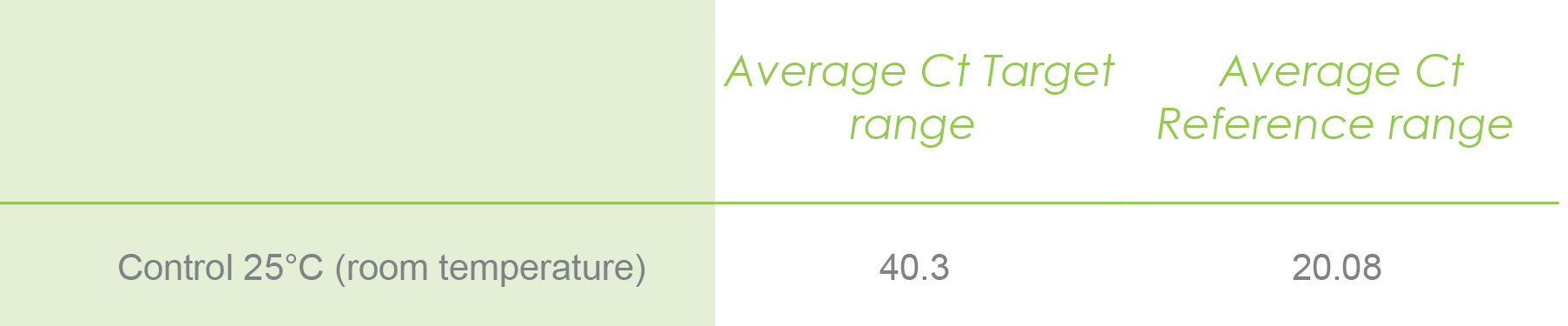
Average Ct target range:
The average Ct target range is the average calculated for all Ct values of plants exposed to control and high-temperature experiments for your target gene.
Average Ct reference range:
The average Ct reference range is the average calculated for all Ct values of plants exposed to control and high-temperature experiments for the reference gene.
Step 2. Calculate the ΔCt individually for each gene per sample
Keep all the values you’ve calculated handy. The next value you’ll want to calculate and add to your list is the individual ΔCt values for each gene per sample.
This is easily accomplished with the following formula.
Formula
ΔCt = Average Ct per sample − Average Ct range
Let me illustrate with the following example. The values in bold are already calculated averages. They are the average for the target and reference genes only for the control.
The rest of the values are Ct values calculated per sample. For instance, the values shown in the next table were calculated only for sample 1 under control and treatment just for illustrative purposes. However, this math should be performed for each sample under control and treatment experiments.
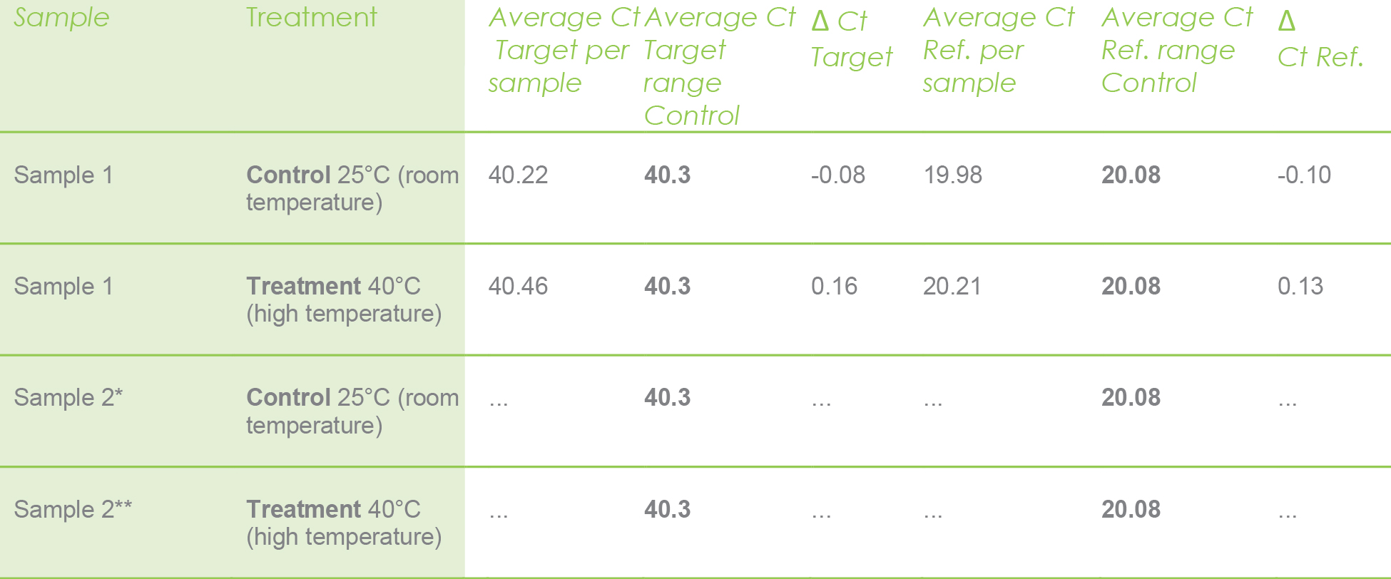
Ref. = Reference gene (actin). * Do the same with all control samples. ** Do the same with all treated samples.
Use the above values only for the sample 1 under control and treatment, calculate with the following formula.
Formula
Ratio = PEC (target)ΔCt(target) / PEC(reference)ΔCt(reference)
Recall, your PEC or primer efficiency was calculated in step 1, shown below.
PEC target: 1.97
PEC reference: 1.95
The ΔCt values for the target and reference are listed below as well.
ΔCt target: 0.13
ΔCt reference: -0.10
Now we can put everything into the equation.
Ratio = 1.970.13 / 1.95-0.10 = 1.13
Here, we have calculated the ratio for the first sample under control and treatment. However, you will need to calculate this ratio for each of your samples and PCR controls too (like the no reverse transcriptase control, as an example).
After that, you will just need to average the ratios for the pool of samples under control and treatment separately.
If the efficiencies are near 100%, (after PEC calculation the value will be 2), the Pfaffl method will give the same result as the Livak method.
In summary, to guide the method selection you should consider:
- Generally acceptable efficiency ranges for analysis (85%-100%)
-Efficiencies appropriate for Livak method 90%-100%
- Efficiencies appropriate for Pfaffl method 85%-100%
Key takeaways
We have a tool that helps you analyze your PCR results using either the Pfaffl or Livak method. This tool has the following calculators all built-in:
This section is used to calculate the PCR Efficiency for your Reference Gene and your Target Gene. The PCR Efficiency is important in order to determine the relative quantification method to use.
This calculator generates the ∆Ct for control and treatment, the ∆∆Ct, and provides you with the expression ratio of your experiment using the Livak Method
This calculator needs the PCR efficiencies in the formula for the target and reference genes. It converts the PCR efficiencies into integer numbers. Then use ∆Ct for control and treatment to calculate the the expression ratio.
You can access to these calculators by clicking this link
Keywords: qPCR, RT-qPCR, gene expression, Ct values, delta Ct.
Bradburn, S. (2019). How To Calculate PCR Primer Efficiencies. In Top Tip Bio. https://toptipbio.com/calculate-primer-efficiencie...
Bradburn, S. (2020). How To Perform The Pfaffl Method For qPCR. In Top Tip Bio. https://toptipbio.com/pfaffl-method-qpcr/
IRIC. (2017). Understanding qPCR results. Institute of Research in Immunology and Cancer (University of Montreal), 1–3.
Kannan, S. (2021). Get the Hang of qPCR Double Delta Ct Analysis in 4 Easy Steps. https://bitesizebio.com/24894/4-easy-steps-to-anal...
Kainz, P. (2000). The PCR plateau phase – towards an understanding of its limitations, Biochimica et Biophysica Acta (BBA) - Gene Structure and Expression, 1494, 23-27. https://doi.org/10.1016/S0167-4781(00)00200-1.
Livak, K. J., & Schmittgen, T. D. (2001). Analysis of relative gene expression data using real-time quantitative PCR and the 2-ΔΔCT method. Methods, 25(4), 402–408. https://doi.org/10.1006/meth.2001.1262
Najafi, M. (2013). How to Analyze Real Time qPCR Data? Biochemistry & Physiology: Open Access, 02(01). https://doi.org/10.4172/2168-9652.1000e114
Pfaffl, M. (2001). A new mathematical model for relative quantification in real-time RT-PCR. Nucleic Acids Research, 29(9), 2002–2007. https://doi.org/10.1111/j.1365-2966.2012.21196.x
Wong, M. L., & Medrano, J. F. (2005). One-Step Versus Two-Step Real- Time PCR. BioTechniques, 39(1), 75–85. https://doi.org/10.2144/05391RV01

Making IPTG stock solution involves weighing out IPTG powder, pouring it into a conical tube or cylinder, and adding deionized water to the desired volume....

IPTG and auto-induction are two ways to induce protein expression in bacteria. They work similarly, but have different trade-offs in terms of convenience. While IPTG...

The final concentration of IPTG used for induction varies from 0.1 to 1.0 mM, with 0.5 or 1.0 mM most frequently used. For proteins with...

A His-tag is a stretch of 6-10 histidine amino acids in a row that is used for affinity purification, protein detection, and biochemical assays. His-tags...